Simple Linear Regression

import numpy as np
import scipy as sp
import pandas as pd
import matplotlib.pyplot as plt
import statsmodels.formula.api as smf

plt.style.use("fivethirtyeight")
import pymc as pm
import seaborn as sns
import arviz as az
from statsmodels.graphics.tsaplots import plot_acf

WARNING (pytensor.tensor.blas): Using NumPy C-API based implementation for BLAS functions.

This is a simple linear regression model as in every textbooks \[ Y_i=\beta_1+\beta_2X_i+u_i\qquad i = 1, 2, ..., n \] where \(Y\) is dependent variable, \(X\) is independent variable and \(u\) is disturbance term. \(\beta_1\) and \(\beta_2\) are unknown parameters that we are aiming to estimate by feeding the data in the model.

Following Gauss-Markov assumptions, \[ E(Y|X_i) = {\beta}_1 + {\beta}_2X_i\\ Y_{i} \sim \mathrm{N}\left({\beta_{1}}+{\beta_{2}}X_{i}, \sigma^{2}\right) \] Similarly, the precision parameter \(h\) is defined as the inverse of variance \(\sigma^2\), i.e. \(h=\frac{1}{\sigma^2}\).

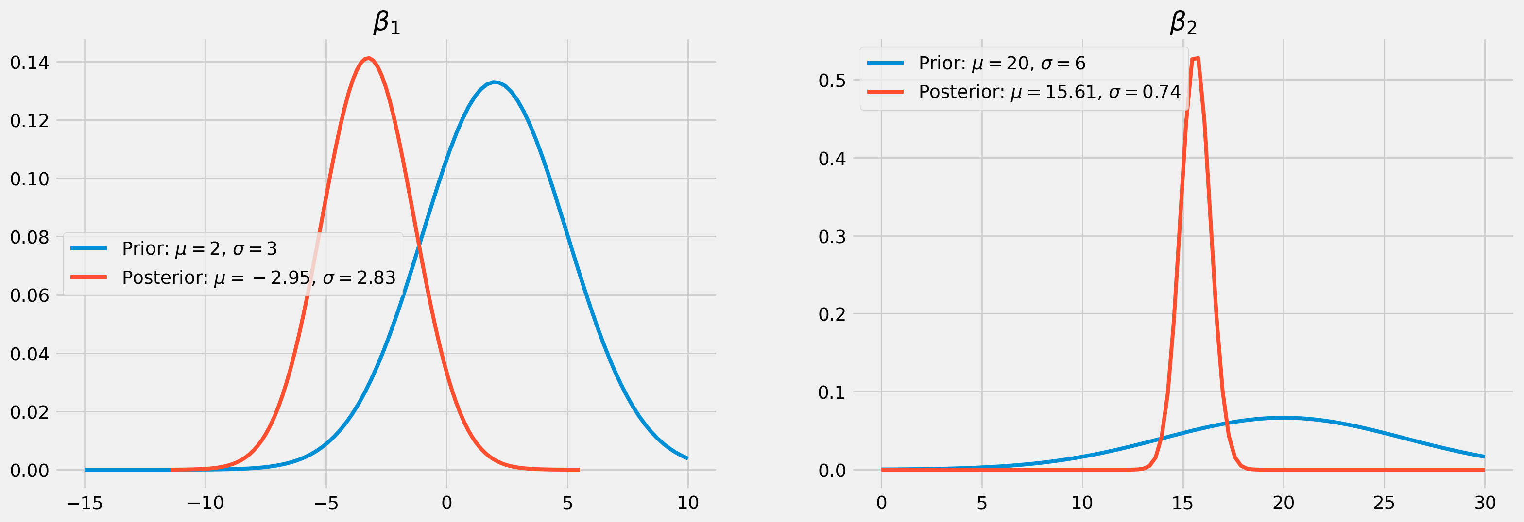
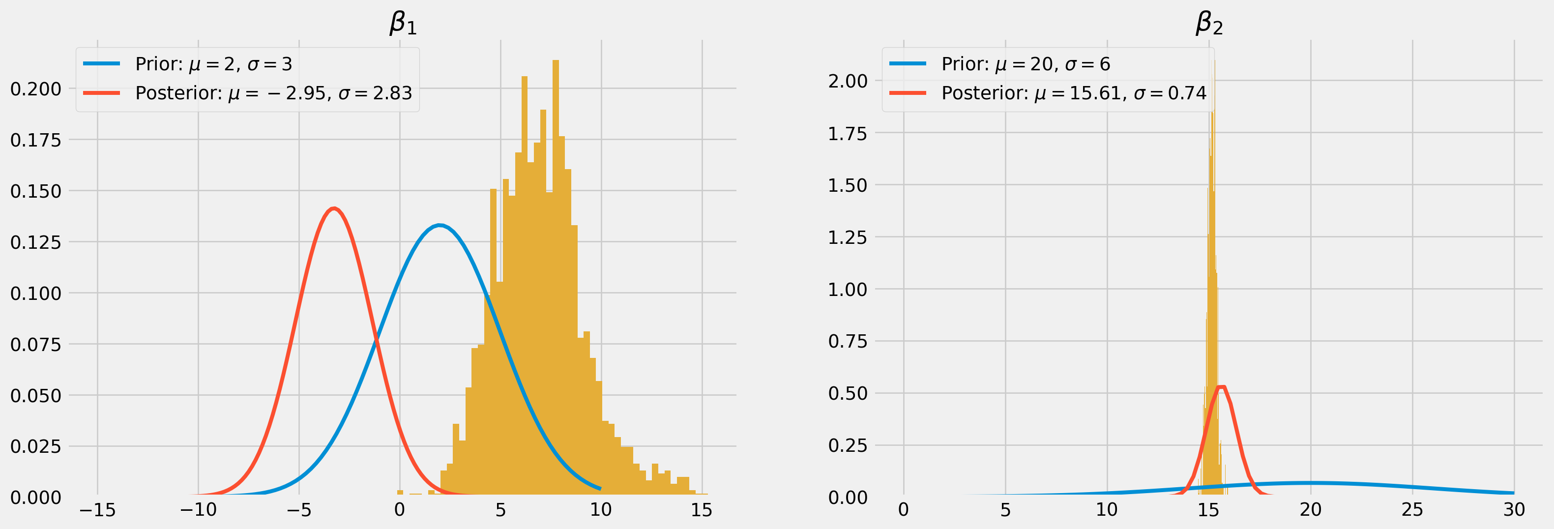
The Priors

Each of these three parameters, i.e. \(\beta_1\), \(\beta_2\) and \(h\) will be estimated, therefore each of them have their own prior elicitation which means defining a prior with all proper knowledge available. For demonstration purpose, we define \(\beta\) priors as normal distributions, however in many case, \(\beta\) and \(h\) are modeled together with a joint distribution.

\[ P(\beta_1)=(2 \pi)^{-\frac{1}{2}} h_1^{\frac{1}{2}} \exp{\left(-\frac{1}{2} h_1 \left(\beta_1-\mu_1\right)^{2}\right)}\\ P(\beta_2)=(2 \pi)^{-\frac{1}{2}} h_2^{\frac{1}{2}} \exp{\left(-\frac{1}{2} h_2 \left(\beta_1-\mu_1\right)^{2}\right)}\\ \]

However the \(h\) can’t be negative, therefore a Gamma distribution would be appropriate. The posterior of \(h\) will follow a Gamma distribution too due to Gamma-Normal conjugate. \[ P(h)=\frac{\theta_{0}^{\alpha_{0}} h^{\alpha_{0}-1} e^{-\theta_{0} h}}{\Gamma\left(\alpha_{0}\right)} \quad 0 \leq h \leq \infty \]

Likelihood Function

With normality assumption, likelihood of \(Y\) is \[ \mathcal{L}\left(Y | \mu_{i}, \sigma^{2}\right)=\prod_{i=1}^n\frac{1}{\sigma \sqrt{2 \pi}} \exp{\left(-\frac{1}{2}\left(\frac{Y_i-\mu_i}{\sigma}\right)^{2}\right)} \]

Equivalently, replace \(\sigma\) by \(h\) and rewrite the function into summation \[ \mathcal{L}\left(Y | \mu_{i}, h\right)=(2 \pi)^{-\frac{n}{2}} h^{\frac{n}{2}} \exp{\left(-\frac{1}{2} h \sum_{i=1}^n\left(Y_{i}-\mu_{i}\right)^{2}\right)} \]

Replace \(\mu_i\) by \({\beta}_1 + {\beta}_2X_i\), note how we have change the notation of parameters \[ \mathcal{L}\left(Y | \beta_1, \beta_2, h\right)=(2 \pi)^{-\frac{n}{2}} h^{\frac{n}{2}} \exp{\left(-\frac{1}{2} h \sum_{i=1}^n\left(Y_{i}-({\beta}_1 + {\beta}_2X_i)\right)^{2}\right)} \]

The likelihood function are the same for \(\beta_1\), \(\beta_2\) and \(h\). \[ \mathcal{L}\left(Y | \beta_1\right)=\mathcal{L}\left(Y | \beta_2\right)=\mathcal{L}\left(Y | h\right)=(2 \pi)^{-\frac{n}{2}} h^{\frac{n}{2}} \exp{\left(-\frac{1}{2} h \sum_{i=1}^n\left(Y_{i}-({\beta}_1 + {\beta}_2X_i)\right)^{2}\right)} \]

The Posteriors

Be careful about the notation, \(h_1\) is the precision of \(\beta_1\) which is a variable rather than a constant viewed in frequentists.

To start from \(\beta_1\) \[ P\left(\beta_{1}\right) \times P\left(Y\mid \beta_{1}\right)=(2 \pi)^{-\frac{1}{2}} h_{1}^{\frac{1}{2}} \exp\left({-\frac{h_{1}}{2}\left(\beta_{1}-\mu_{1}\right)^{2}}\right) \times (2 \pi)^{-\frac{n}{2}} h^{\frac{n}{2}} \exp{\left(-\frac{1}{2} h \sum_{i=1}^n\left(Y_{i}-({\beta}_1 + {\beta}_2X_i)\right)^{2}\right)} \]

Join terms \[ P\left(\beta_{1}\right) \times P\left(Y\mid \beta_{1}\right)=(2 \pi)^{-\frac{n+1}{2}} h_{1}^{\frac{1}{2}} h^{\frac{n}{2}} \exp{\left(-\frac{1}{2} h_{1}\left(\beta_{1}-\mu_{1}\right)^{2}-\frac{1}{2} h \sum_{i=1}^n\left(Y_{i}-\beta_{1}-\beta_{2} X_{i}\right)^{2}\right)} \]

Let’s focus on exponential term for now, expand the brackets \[\begin{align} &\exp{\left(-\frac{1}{2} h_{1}\left(\beta_{1}-\mu_{1}\right)^{2}-\frac{1}{2} h \sum_{i=1}^n\left(Y_{i}-\beta_{1}-\beta_{2} X_{i}\right)^{2}\right)}\\ &= \exp{\left[-\frac{1}{2} h_{1}\left(\beta_{1}^{2}-2 \beta_{1} \mu_{1}+\mu_{1}^{2}\right)-\frac{1}{2} h\left(n \beta_{1}^{2}-2 \beta_{1} \sum_{i=1}^n\left(Y_{i}-\beta_{2} X_{i}\right)+\sum_{i=1}^n\left(Y_{i}-\beta_{2} X_{i}\right)^{2}\right)\right]}\\ &=\exp{\left[-\frac{1}{2}\left(h_{1}+n h\right) \beta_{1}^{2}-\frac{1}{2}\left[-2 h_{1} \mu_{1}-2 h \sum_{i=1}^n\left(Y_{i}-\beta_{2} X_{i}\right)\right] \beta_{1}-\frac{1}{2} h_{1} \mu_{1}^{2}-\frac{1}{2} h \sum_{i=1}^n\left(Y_{i}-\beta_{2} X_{i}\right)^{2}\right]}\\ &=\exp{\left[-\frac{1}{2}\left(h_{1}+n h\right) \beta_{1}^{2}+\left[h_{1} \mu_{1}+h \sum_{i=1}^n\left(Y_{i}-\beta_{2} X_{i}\right)\right] \beta_{1}+\frac{-\frac{1}{2}\left[h_{1} \mu_{1}+h \sum_{i=1}^n\left(Y_{i}-\beta_{2} X_{i}\right)\right]^{2}}{h_{1}+n h}-\frac{-\frac{1}{2}\left[h_{1} \mu_{1}+h \sum_{i=1}^n\left(Y_{i}-\beta_{2} X_{i}\right)\right]^{2}}{h_{1}+n h}-\frac{1}{2} h_{1} \mu_{1}^{2}-\frac{1}{2} h \sum_{i=1}^n\left(Y_{i}-\beta_{2} X_{i}\right)^{2}\right]}\\ \end{align}\] The first three terms can be combined and the rest are free of \(\beta_1\), which will be denoted as \(C\).

\[ -\frac{1}{2} \left(h_{1}+n h\right)\left[\beta_{1}-\frac{\left(h_{1} \mu_{1}+h \sum_{i=1}^n\left(Y_{i}-\beta_{2} X_{i}\right)\right)}{h_{1}+n h}\right]^{2} \]

Back to Bayes’ Theorem \[ P\left(\beta_{1} | Y\right)=\frac{(2 \pi)^{-\frac{n+1}{2}} h_{1}^{\frac{1}{2}} h^{\frac{n}{2}} \exp{\left[-\frac{1}{2}\left(h_{1}+n h\right)\left[\beta_{1}-\frac{\left(h_{1} \mu_{1}+h \sum_{i=1}^n\left(Y_{i}-\beta_{2} X_{i}\right)\right)}{h_{1}+n h}\qquad\right]^{2}+C\right]}}{\int_{-\infty}^{\infty}(2 \pi)^{-\frac{n+1}{2}} h_{1}^{\frac{1}{2}} h^{\frac{n}{2}} \exp{\left[-\frac{1}{2}\left(h_{1}+n h\right)\left[u-\frac{\left(h_{1} \mu_{1}+h \sum_{i=1}^n\left(Y_{i}-\beta_{2} X_{i}\right)\right)}{h_{1}+n h}\qquad\right]^{2}+C\right]} d u} \]

Cancel out terms, we obtain \[ P\left(\beta_{1} | Y\right)=\frac{\exp{\left[-\frac{1}{2}\left(h_{1}+n h\right)\left[\beta_{1}-\frac{\left(h_{1} \mu_{1}+h \sum_{i=1}^n\left(Y_{i}-\beta_{2} X_{i}\right)\right)}{h_{1}+n h}\qquad\right]^{2}\right]}}{\int_{-\infty}^{\infty} \exp{\left[-\frac{1}{2}\left(h_{1}+n h\right)\left[u-\frac{\left(h_{1} \mu_{1}+h \sum_{i=1}^n\left(Y_{i}-\beta_{2} X_{i}\right)\right)}{h_{1}+n h}\qquad\right]^{2}\right]} d u} \]

Now multiply both numerator and denominator by \[ \frac{\sqrt{h_{1}+n h}}{\sqrt{2 \pi}} \] which yields

\[ P\left(\beta_{1} | Y\right)=\frac{\frac{\sqrt{h_{1}+n h}}{\sqrt{2 \pi}}\exp{\left[-\frac{1}{2}\left(h_{1}+n h\right)\left[\beta_{1}-\frac{\left(h_{1} \mu_{1}+h \sum_{i=1}^n\left(Y_{i}-\beta_{2} X_{i}\right)\right)}{h_{1}+n h}\qquad\right]^{2}\right]}}{\int_{-\infty}^{\infty}\frac{\sqrt{h_{1}+n h}}{\sqrt{2 \pi}} \exp{\left[-\frac{1}{2}\left(h_{1}+n h\right)\left[u-\frac{\left(h_{1} \mu_{1}+h \sum_{i=1}^n\left(Y_{i}-\beta_{2} X_{i}\right)\right)}{h_{1}+n h}\qquad\right]^{2}\right]} d u} \]

The denominator is equal to \(1\), which leaves us \[ P\left(\beta_{1} | Y\right)=(2\pi)^{-\frac{1}{2}}(h_1+nr)^{\frac{1}{2}}\exp{\left[-\frac{1}{2}\left(h_{1}+n h\right)\left[\beta_{1}-\frac{\left(h_{1} \mu_{1}+h \sum_{i=1}^n\left(Y_{i}-\beta_{2} X_{i}\right)\right)}{h_{1}+n h}\qquad\right]^{2}\right]} \] Compare with the prior \[ P(\beta_1)=(2 \pi)^{-\frac{1}{2}} h_1^{\frac{1}{2}} \exp{\left(-\frac{1}{2} h_1 \left(\beta_1-\mu_1\right)^{2}\right)} \]

The posterior hyperparameters of \(\beta_1\) are \[ \begin{gathered} \mu_{\text {1posterior }}=\frac{h_{1} \mu_{1}+h \sum_{i=1}^n\left(Y_{i}-\beta_{2} X_{i}\right)}{h_{1}+n h} \\ h_{\text {1posterior }}=h_{1}+n h \end{gathered} \]

def mu_tau_1_post(tau_1_prior, mu_1_prior, mu_2_prior, tau_lh, Y, X, n):
    mu_1_post = (tau_1_prior * mu_1_prior + tau_lh * (np.sum(Y - mu_2_prior * X))) / (
        tau_1_prior + n * tau_lh
    )
    tau_1_post = tau_1_prior + n * tau_lh
    sigma_1_post = 1 / np.sqrt(tau_1_post)
    return mu_1_post, tau_1_post, sigma_1_post

The derivation of posterior for \(\beta_2\) are very, will not be reproduced here \[ \begin{gathered} \mu_{2 \text { posterior }}=\frac{h_{2} \mu_{2}+h \sum_{i=1}^n X_{i}\left(Y_{i}-\beta_{1}\right)}{h_{2}+h \sum_{i=1}^n X_{i}^{2}} \\ h_{2 \text { posterior }}=h_{2}+h \sum_{i=1}^n X_{i}^{2} \end{gathered} \]

def mu_tau_2_post(tau_2_prior, mu_2_prior, mu_1_prior, tau_lh, Y, X, n):
    mu_2_post = (tau_2_prior * mu_2_prior + tau_lh * np.sum(X * (Y - mu_1_prior))) / (
        tau_2_prior + tau_lh * np.sum(X**2)
    )
    tau_2_post = tau_2_prior + tau_lh * np.sum(X**2)
    sigma_2_post = 1 / np.sqrt(tau_2_post)
    return mu_2_post, tau_2_post, sigma_2_post

We will derive the posterior of \(h\), prior multiply by likelihood equals \[ P(h) P(Y | h)=\frac{\beta_{0}^{\alpha_{0}} h^{\alpha_{0}-1} e^{-\beta_{0} h}}{\Gamma\left(\alpha_{0}\right)} *(2 \pi)^{-\frac{n}{2}} h^{\frac{n}{2}} \exp{\left[-\frac{1}{2} h \Sigma\left(y_{i}-\left(b_{0}-b_{1} x_{i}\right)\right)^{2}\right]} \]

However, please note that there is no need to memorize any of these derivations, they are here as a reference. We don’t run regression based on these formulae.

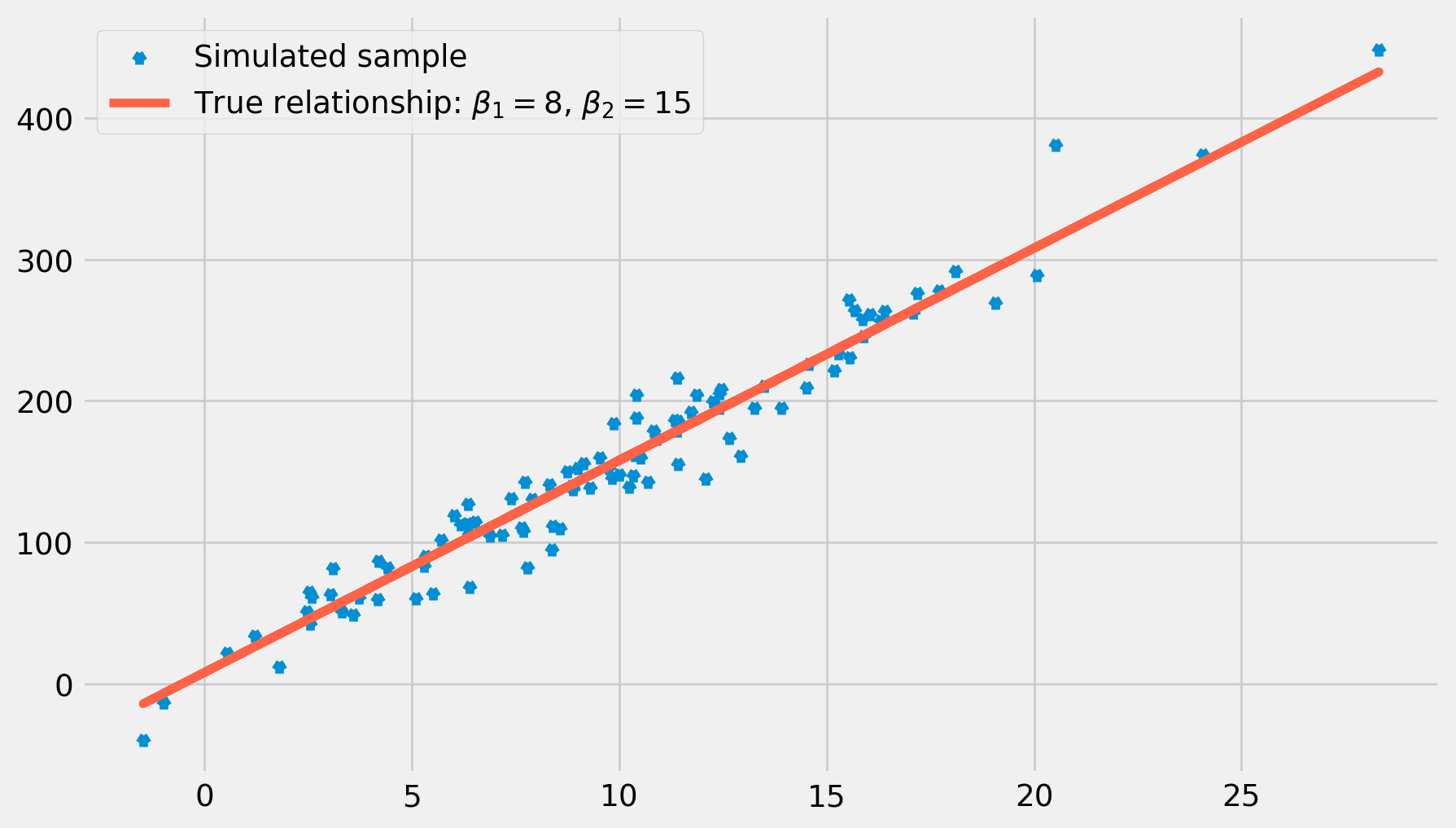
A Simulated Example

Generate the sample with the real relationship \[ Y_i = 8+15X_i+u_i \]

beta_1, beta_2 = 8, 15
n = 100
X = sp.stats.norm(loc=10, scale=5).rvs(size=n)
u = np.random.randn(n) * 20
Y_hat = beta_1 + beta_2 * X
Y = Y_hat + u

data = pd.DataFrame(dict(X=X, Y=Y, Y_hat=Y_hat))
fig, ax = plt.subplots(figsize=(10, 6))
ax.scatter(data["X"], data["Y"], marker="1", label="Simulated sample")
ax.plot(
    data["X"],
    data["Y_hat"],
    color="tomato",
    label=r"True relationship: $\beta_1={}$, $\beta_2={}$".format(beta_1, beta_2),
)
ax.legend()
plt.show()

mu_1_prior, sigma_1_prior = 2, 3
mu_2_prior, sigma_2_prior = 20, 6
sigma_lh = np.std(Y)
tau_lh = 1 / sigma_lh**2
tau_1_prior, tau_2_prior = 1 / sigma_1_prior**2, 1 / sigma_2_prior**2

mu_1_post, tau_1_post, sigma_1_post = mu_tau_1_post(
    tau_1_prior, mu_1_prior, mu_2_prior, tau_lh, Y, X, n
)
mu_2_post, tau_2_post, sigma_2_post = mu_tau_2_post(
    tau_2_prior, mu_2_prior, mu_1_prior, tau_lh, Y, X, n
)
betax_prior_1 = np.linspace(-15, 10, 100)
betax_prior_2 = np.linspace(0, 30, 100)

betay_prior_1 = sp.stats.norm.pdf(betax_prior_1, loc=mu_1_prior, scale=sigma_1_prior)
betay_prior_2 = sp.stats.norm.pdf(betax_prior_2, loc=mu_2_prior, scale=sigma_2_prior)

betax_post_1 = np.linspace(
    mu_1_post - 3 * sigma_1_post, mu_1_post + 3 * sigma_1_post, 100
)
betax_post_2 = np.linspace(mu_2_post - sigma_2_post, mu_2_post + sigma_2_post, 100)

betay_post_1 = sp.stats.norm.pdf(betax_prior_1, loc=mu_1_post, scale=sigma_1_post)
betay_post_2 = sp.stats.norm.pdf(betax_prior_2, loc=mu_2_post, scale=sigma_2_post)

fig, ax = plt.subplots(figsize=(18, 6), nrows=1, ncols=2)
ax[0].plot(
    betax_prior_1,
    betay_prior_1,
    lw=3,
    label=r"Prior: $\mu={}$, $\sigma={}$".format(mu_1_prior, sigma_1_prior),
)
ax[0].plot(
    betax_post_1,
    betay_post_1,
    lw=3,
    label=r"Posterior: $\mu={:.2f}$, $\sigma={:.2f}$".format(mu_1_post, sigma_1_post),
)
ax[0].set_title(r"$\beta_1$")
ax[1].plot(
    betax_prior_2,
    betay_prior_2,
    lw=3,
    label=r"Prior: $\mu={}$, $\sigma={}$".format(mu_2_prior, sigma_2_prior),
)
ax[1].plot(
    betax_prior_2,
    betay_post_2,
    lw=3,
    label=r"Posterior: $\mu={:.2f}$, $\sigma={:.2f}$".format(mu_2_post, sigma_2_post),
)
ax[1].set_title(r"$\beta_2$")
ax[0].legend()
ax[1].legend(loc="upper left")

# print('mu_1_post: {:.4f}'.format(mu_1_post))  depends on you if you'd like to print them
# print('tau_1_post: {:.10f}'.format(tau_1_post))
# print('sigma_1_post: {:.4f}'.format(sigma_1_post))
# print('')
# print('mu_2_post: {:.4f}'.format(mu_2_post))
# print('tau_2_post: {:.10f}'.format(tau_2_post))
# print('sigma_2_post: {:.4f}'.format(sigma_2_post))
plt.show()

with pm.Model() as linreg_model:  # model specifications in pymc are wrapped in a with-statement
    # Define priors
    beta1_hat = pm.Normal("beta1_hat", mu=8, sigma=3)
    beta2_hat = pm.Normal("beta2_hat", mu=15, sigma=0.5)
    sigma = pm.Gamma("sigma", alpha=2, beta=1)

    # Define likelihood
    Y_hat = pm.Deterministic("Y_hat", beta1_hat + beta2_hat * X)
    Y_lh = pm.Normal("Y_lh", mu=Y_hat, sigma=sigma, observed=Y)

    # Sampling
    start = pm.Metropolis()
    trace = pm.sample(2000, cores=1, step=start, return_inferencedata=True)

Sequential sampling (2 chains in 1 job)
CompoundStep
>Metropolis: [beta1_hat]
>Metropolis: [beta2_hat]
>Metropolis: [sigma]

/home/runner/.cache/pypoetry/virtualenvs/workspace-env-xqASYfE0-py3.12/lib/python3.12/site-packages/pymc/step_metho
ds/metropolis.py:285: RuntimeWarning:

overflow encountered in exp

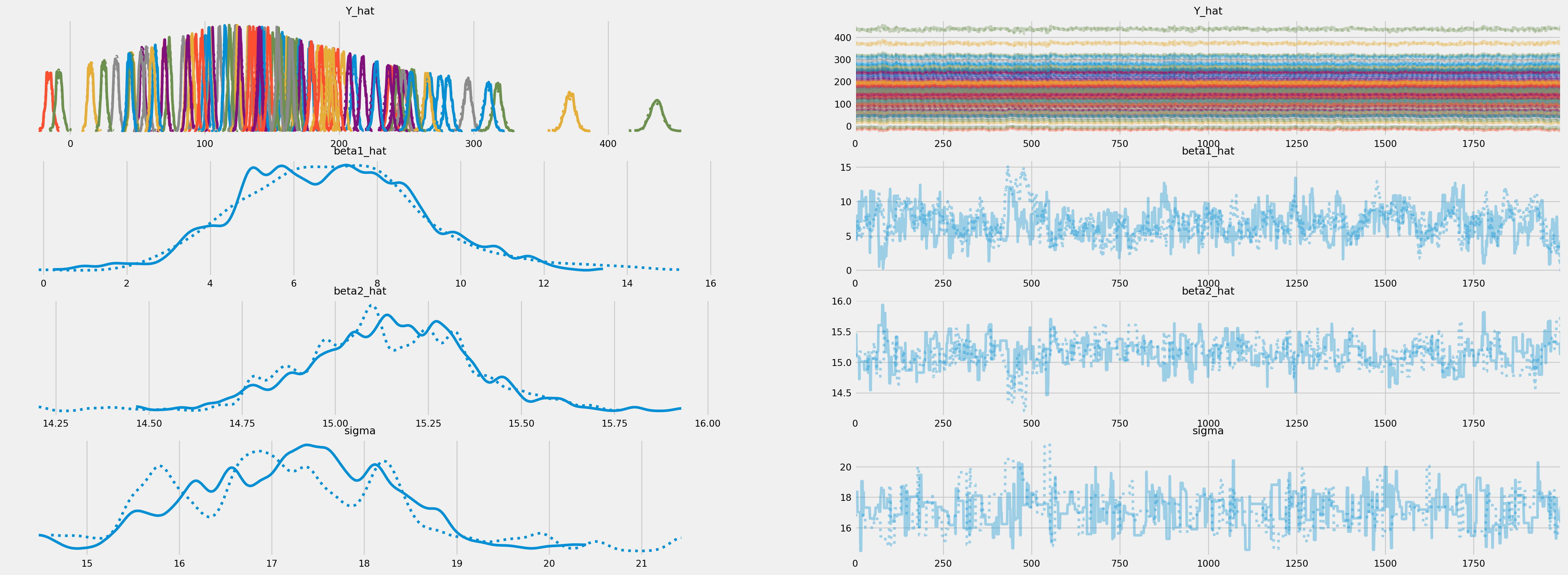
Sampling 2 chains for 1_000 tune and 2_000 draw iterations (2_000 + 4_000 draws total) took 3 seconds.
We recommend running at least 4 chains for robust computation of convergence diagnostics
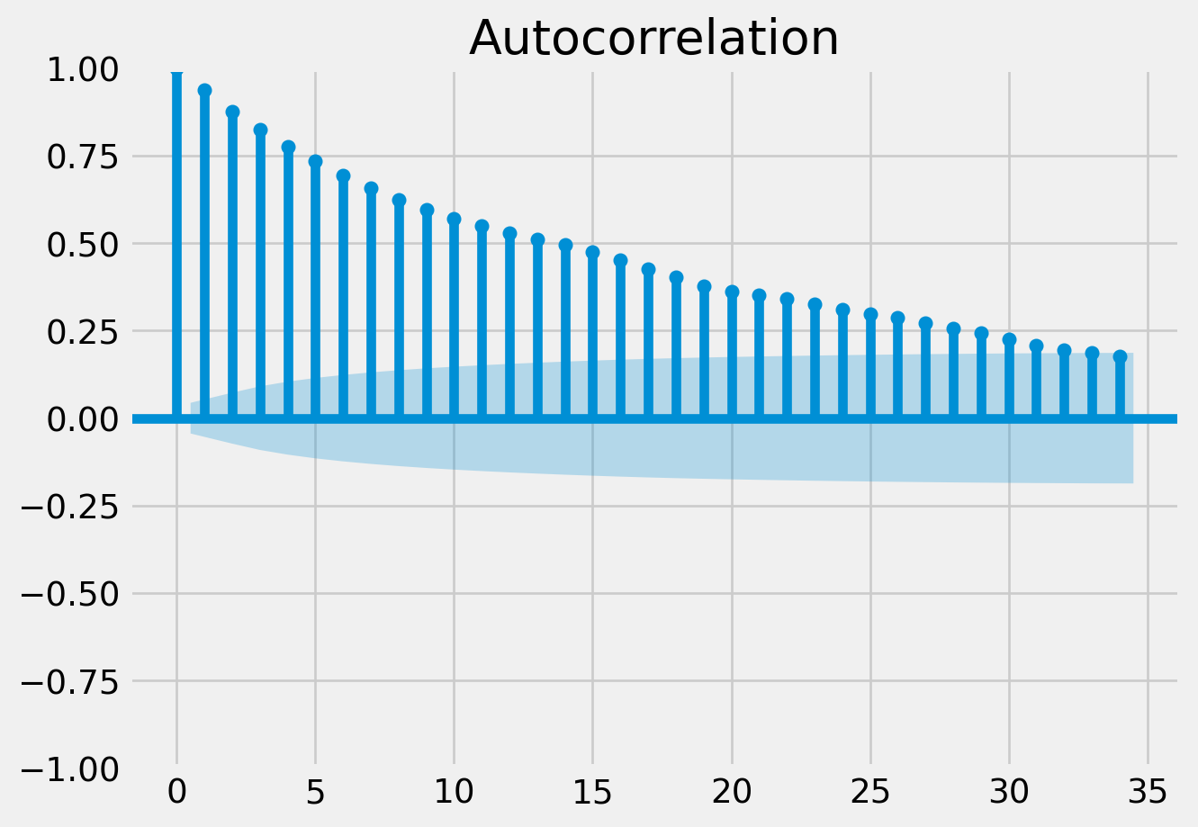
The rhat statistic is larger than 1.01 for some parameters. This indicates problems during sampling. See https://arxiv.org/abs/1903.08008 for details
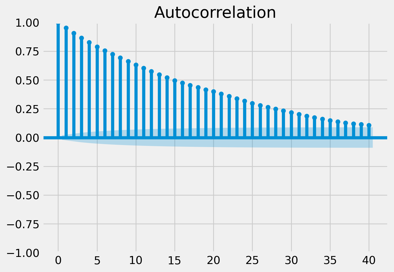
The effective sample size per chain is smaller than 100 for some parameters.  A higher number is needed for reliable rhat and ess computation. See https://arxiv.org/abs/1903.08008 for details

az.plot_trace(trace, figsize=(27, 10), compact=True)
plt.show()

fig, ax = plt.subplots(figsize=(12, 7))
ax.scatter(X, Y, marker="1")

beta1_chain, beta2_chain = (
    trace.posterior.beta1_hat.data[1],
    trace.posterior.beta2_hat.data[1],
)
beta1_m = np.mean(beta1_chain)
beta2_m = np.mean(beta2_chain)

draws = range(0, len(trace.posterior.beta1_hat.data[1]), 10)
ax.plot(
    X, beta1_chain[draws] + beta2_chain[draws] * X[:, np.newaxis], c="gray", alpha=0.3
)

ax.plot(
    X,
    beta1_m + beta2_m * X,
    c="k",
    label=r"Y = {:.2f} + {:.2f} X".format(beta1_m, beta2_m),
)

ax.set_xlabel("X")
ax.set_ylabel("Y")
ax.legend()
plt.show()

fig, ax = plt.subplots(figsize=(18, 6), nrows=1, ncols=2)
ax[0].plot(
    betax_prior_1,
    betay_prior_1,
    lw=3,
    label=r"Prior: $\mu={}$, $\sigma={}$".format(mu_1_prior, sigma_1_prior),
)
ax[0].plot(
    betax_post_1,
    betay_post_1,
    lw=3,
    label=r"Posterior: $\mu={:.2f}$, $\sigma={:.2f}$".format(mu_1_post, sigma_1_post),
)
ax[0].hist(trace.posterior.beta1_hat.data[1], density=True, bins=50)
ax[0].set_title(r"$\beta_1$")


ax[1].plot(
    betax_prior_2,
    betay_prior_2,
    lw=3,
    label=r"Prior: $\mu={}$, $\sigma={}$".format(mu_2_prior, sigma_2_prior),
)
ax[1].plot(
    betax_prior_2,
    betay_post_2,
    lw=3,
    label=r"Posterior: $\mu={:.2f}$, $\sigma={:.2f}$".format(mu_2_post, sigma_2_post),
)
ax[1].set_title(r"$\beta_2$")
ax[1].hist(trace.posterior.beta2_hat.data[0], density=True, bins=50)
ax[0].legend()
ax[1].legend(loc="upper left")

plt.show()

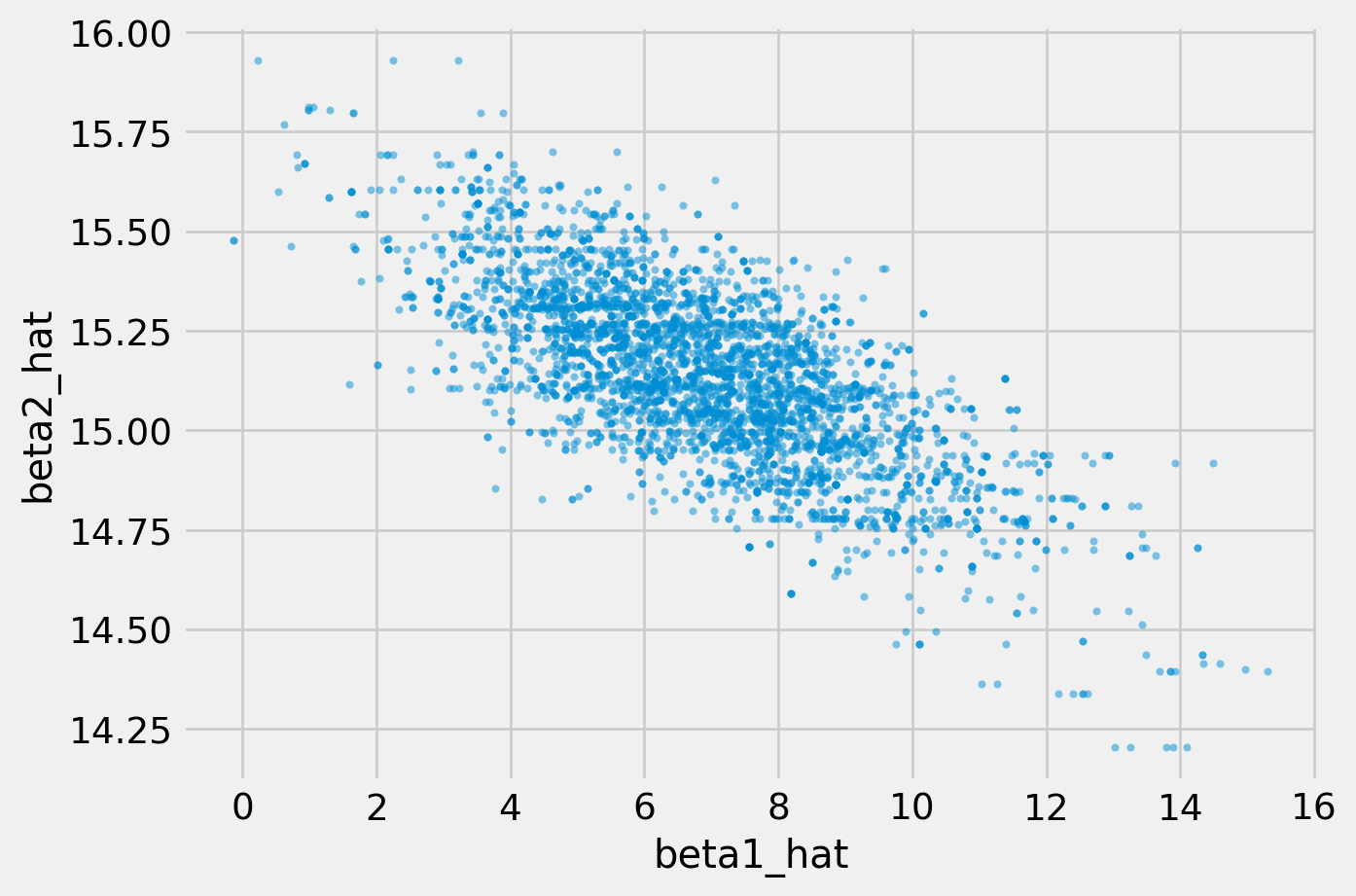
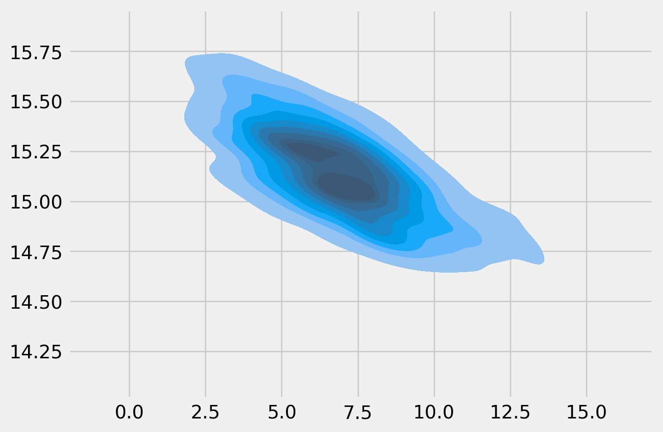
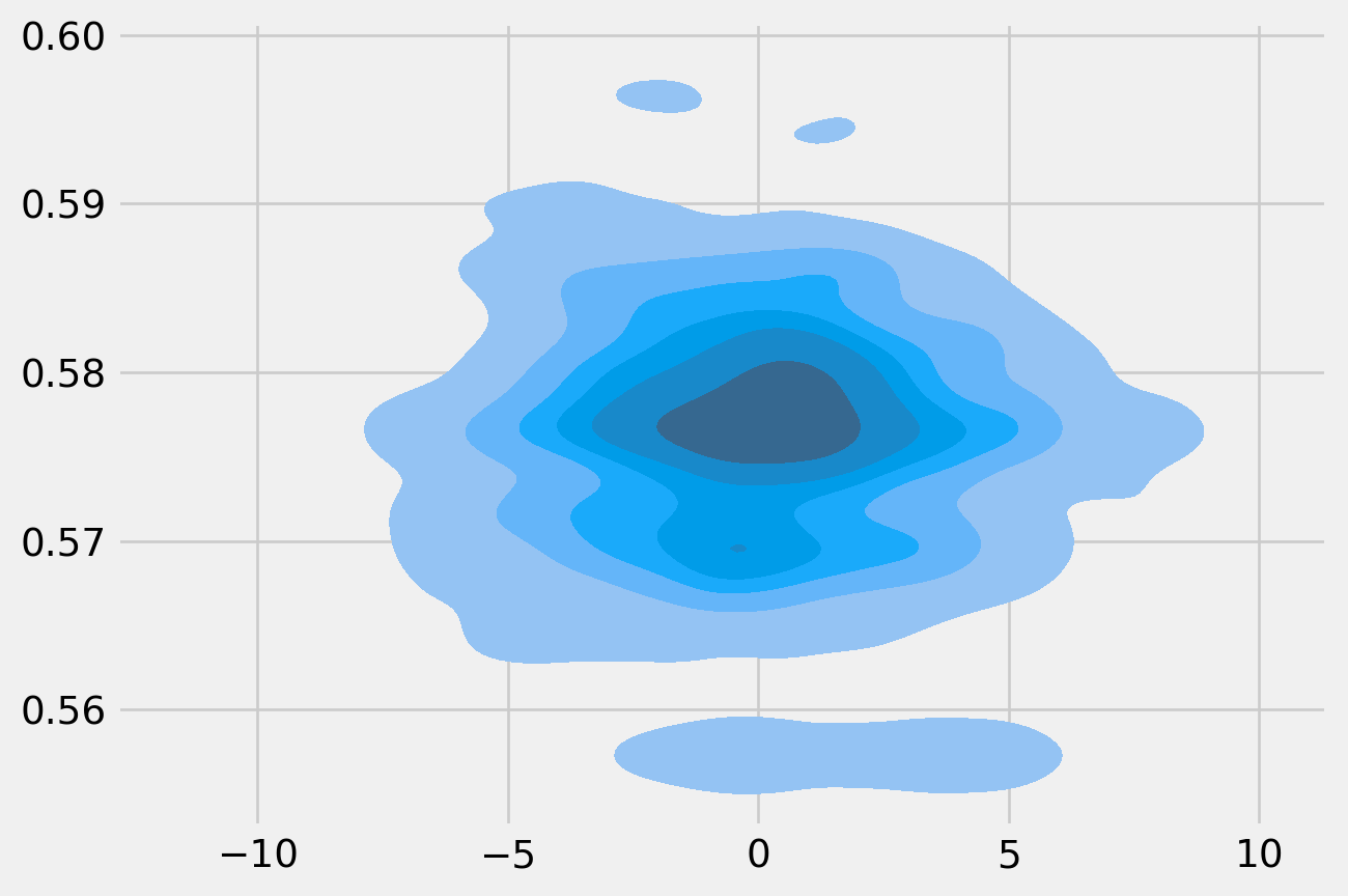
By plotting the scatter plot of simulated \(\beta_1\) and \(\beta_2\), we actually can see the joint of posterior of them, which is by default a ellipsoid.

az.plot_pair(trace, var_names=["beta1_hat", "beta2_hat"], scatter_kwargs={"alpha": 0.5})
plt.show()

sns.kdeplot(
    x=trace.posterior.beta1_hat.data[1], y=trace.posterior.beta2_hat.data[1], fill=True
)
plt.show()

x = plot_acf(trace.posterior.beta1_hat.data[1])

An Example of Apartment Price

df = pd.read_excel("Basic_Econometrics_practice_data.xlsx", "CN_Cities_house_price")

df.head()

	cities	house_price	salary
0	Shenzhen	87957	64878
1	Beijing	64721	69434
2	Shanghai	59072	72232
3	Xiamen	49803	58140
4	Guangzhou	39851	68304

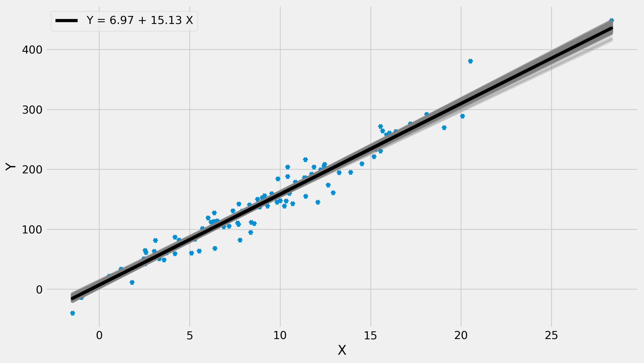
The model to fit the data ill be exactly as we derived above, i.e. \[ Y_i=\beta_1+\beta_2X_i+u_i\qquad i = 1, 2, ..., n \]

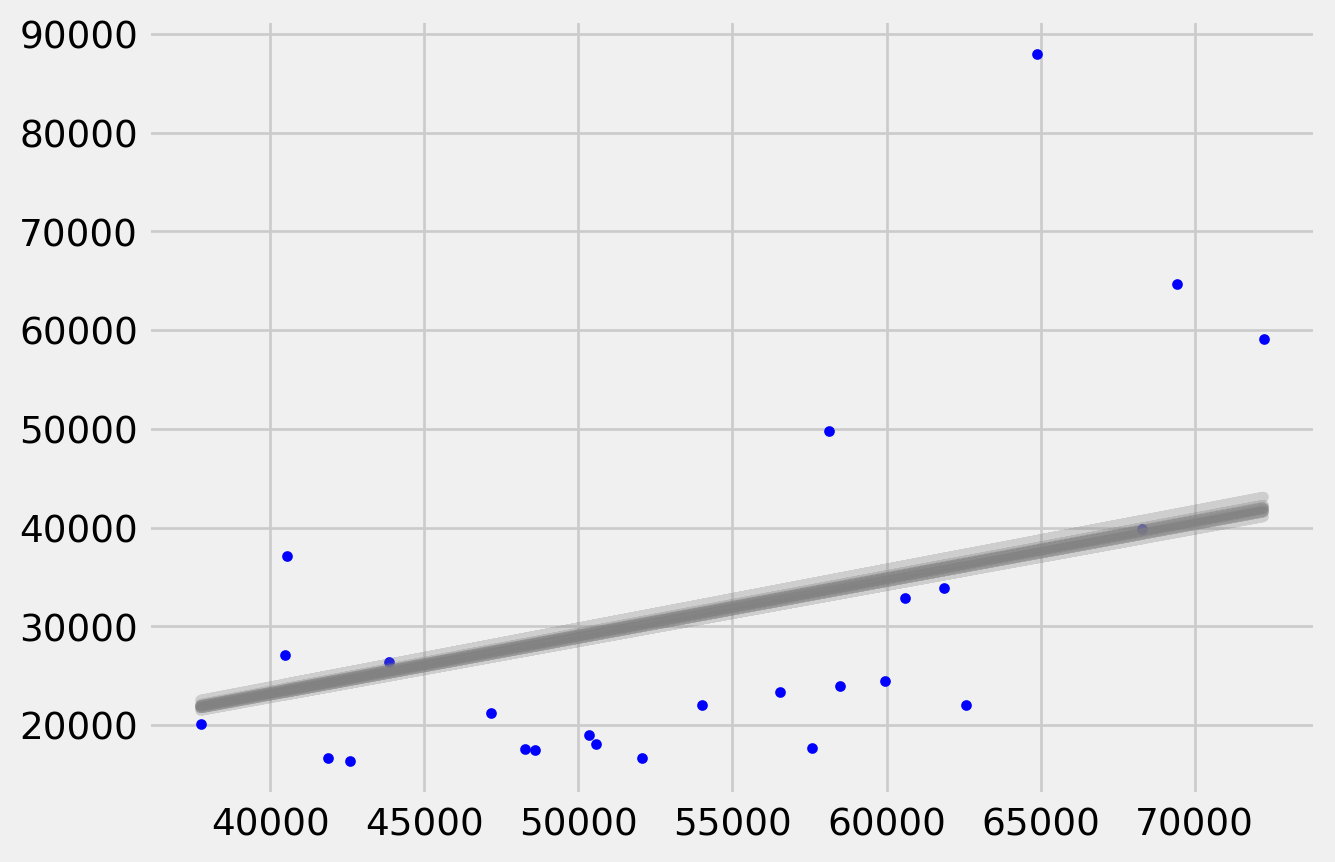
This simple model aims to explain the influence of salary on apartment price per square meter. The \(\beta_1\) doesn’t have much meaning in the model, literally it means the apartment price when salary equals \(0\). However \(\beta_2\) has a concrete meaning that how much apartment price can raise based on every one yuan increase in average salary.

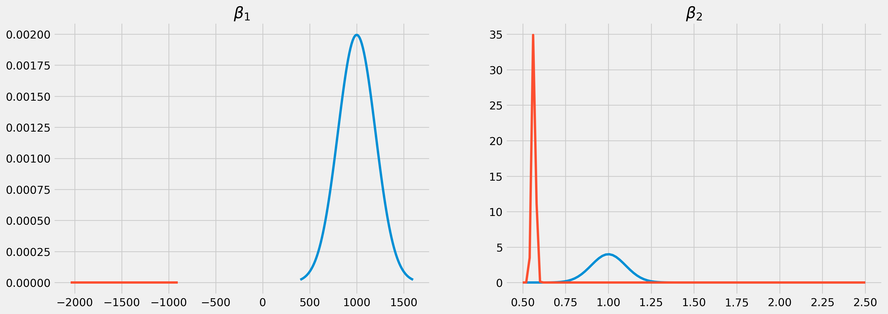
We can choose to elicit priors’ hyperparameters for \(\beta_1\) and \(\beta_2\) as \[ \mu_1 = 1000\\ \sigma_1 = 200 \qquad h_1 = \frac{1}{\sigma_1^2}\\ \mu_2 = 1.5\\ \sigma_2 = .3 \qquad h_2 = \frac{1}{\sigma_2^2}\\ \]

Y, X = df["house_price"], df["salary"]

mu_1_prior, sigma_1_prior = 1000, 200
mu_2_prior, sigma_2_prior = 1, 0.1
sigma_lh = 3000
tau_lh = 1 / sigma_lh**2
tau_1_prior, tau_2_prior = 1 / sigma_1_prior**2, 1 / sigma_2_prior**2

betax_prior_1 = np.linspace(400, 1600, 100)
betax_prior_2 = np.linspace(0.5, 2.5, 100)

betay_prior_1 = sp.stats.norm.pdf(betax_prior_1, loc=mu_1_prior, scale=sigma_1_prior)
betay_prior_2 = sp.stats.norm.pdf(betax_prior_2, loc=mu_2_prior, scale=sigma_2_prior)
n = len(X)

# use functions to calculate posterior hyperparameters
mu_1_post, tau_1_post, sigma_1_post = mu_tau_1_post(
    tau_1_prior, mu_1_prior, mu_2_prior, tau_lh, Y, X, n
)
mu_2_post, tau_2_post, sigma_2_post = mu_tau_2_post(
    tau_2_prior, mu_2_prior, mu_1_prior, tau_lh, Y, X, n
)

betay_post_1 = sp.stats.norm.pdf(betax_prior_1, loc=mu_1_post, scale=sigma_1_post)
betay_post_2 = sp.stats.norm.pdf(betax_prior_2, loc=mu_2_post, scale=sigma_2_post)


fig, ax = plt.subplots(figsize=(17, 6), nrows=1, ncols=2)

betax_post_1 = np.linspace(
    mu_1_post - 3 * sigma_1_post, mu_1_post + 3 * sigma_1_post, 100
)
# betax_post_2 = np.linspace(mu_2_post-sigma_2_post, mu_2_post+sigma_2_post, 100)

ax[0].plot(betax_prior_1, betay_prior_1, lw=3)
ax[0].plot(betax_post_1, betay_post_1, lw=3)
ax[0].set_title(r"$\beta_1$")
ax[1].plot(betax_prior_2, betay_prior_2, lw=3)
ax[1].plot(betax_prior_2, betay_post_2, lw=3)
ax[1].set_title(r"$\beta_2$")

plt.show()

print("mu_1_post: {:.4f}".format(mu_1_post))
print("tau_1_post: {:.10f}".format(tau_1_post))
print("sigma_1_post: {:.4f}".format(sigma_1_post))
print("")
print("mu_2_post: {:.4f}".format(mu_2_post))
print("tau_2_post: {:.10f}".format(tau_2_post))
print("sigma_2_post: {:.4f}".format(sigma_2_post))

mu_1_post: -1473.2840
tau_1_post: 0.0000277778
sigma_1_post: 189.7367

mu_2_post: 0.5640
tau_2_post: 8442.1727574444
sigma_2_post: 0.0109

model = smf.ols(formula="house_price ~ salary", data=df)
results = model.fit()
print(results.summary())

                            OLS Regression Results                            
==============================================================================
Dep. Variable:            house_price   R-squared:                       0.365
Model:                            OLS   Adj. R-squared:                  0.337
Method:                 Least Squares   F-statistic:                     13.21
Date:                Fri, 13 Sep 2024   Prob (F-statistic):            0.00139
Time:                        08:55:58   Log-Likelihood:                -274.08
No. Observations:                  25   AIC:                             552.2
Df Residuals:                      23   BIC:                             554.6
Df Model:                           1                                         
Covariance Type:            nonrobust                                         
==============================================================================
                 coef    std err          t      P>|t|      [0.025      0.975]
------------------------------------------------------------------------------
Intercept  -2.918e+04   1.66e+04     -1.758      0.092   -6.35e+04    5156.201
salary         1.1010      0.303      3.635      0.001       0.474       1.728
==============================================================================
Omnibus:                       14.403   Durbin-Watson:                   0.926
Prob(Omnibus):                  0.001   Jarque-Bera (JB):               14.263
Skew:                           1.457   Prob(JB):                     0.000800
Kurtosis:                       5.280   Cond. No.                     3.12e+05
==============================================================================

Notes:
[1] Standard Errors assume that the covariance matrix of the errors is correctly specified.
[2] The condition number is large, 3.12e+05. This might indicate that there are
strong multicollinearity or other numerical problems.

ols_coeff = pd.DataFrame(results.params, columns=["OLS estimates"])
ols_coeff

	OLS estimates
Intercept	-29181.169815
salary	1.100985

with pm.Model() as model:  # model specifications in pymc are wrapped in a with-statement
    # Define priors
    beta1_hat = pm.Normal("beta1_hat", mu=0, sigma=3)
    beta2_hat = pm.Normal("beta2_hat", mu=0, sigma=0.5)
    sigma = pm.Gamma("sigma", alpha=2, beta=1)

    # Define likelihood
    Y_lh = pm.Normal(
        "Y_lh", mu=beta1_hat + beta2_hat * X.values, sigma=sigma, observed=Y.values
    )

    # Sampling
    start = pm.Metropolis()
    trace = pm.sample(10000, cores=1, step=start, return_inferencedata=True)

Sequential sampling (2 chains in 1 job)
CompoundStep
>Metropolis: [beta1_hat]
>Metropolis: [beta2_hat]
>Metropolis: [sigma]

/home/runner/.cache/pypoetry/virtualenvs/workspace-env-xqASYfE0-py3.12/lib/python3.12/site-packages/pymc/step_metho
ds/metropolis.py:285: RuntimeWarning:

overflow encountered in exp

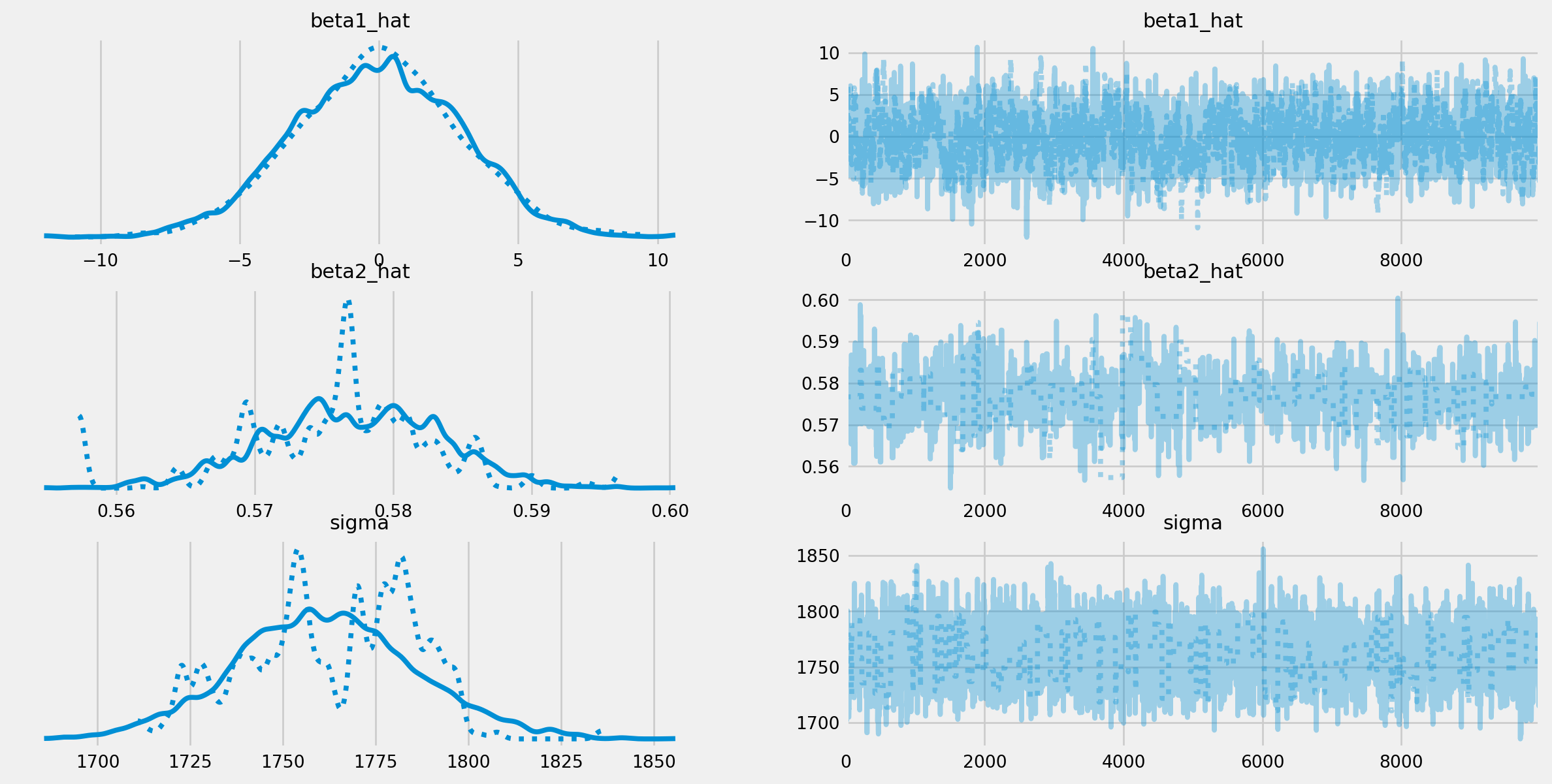
Sampling 2 chains for 1_000 tune and 10_000 draw iterations (2_000 + 20_000 draws total) took 11 seconds.
We recommend running at least 4 chains for robust computation of convergence diagnostics
The rhat statistic is larger than 1.01 for some parameters. This indicates problems during sampling. See https://arxiv.org/abs/1903.08008 for details

fig, ax = plt.subplots(figsize=(18, 6), nrows=1, ncols=2)
ax[0].hist(trace.posterior.beta1_hat.data[1], density=True, bins=100)
ax[0].set_title(r"$\beta_1$")
ax[1].set_title(r"$\beta_2$")
ax[1].hist(trace.posterior.beta2_hat.data[0], density=True, bins=100)

plt.show()

az.plot_trace(trace, figsize=(14, 7))
plt.show()

x = plot_acf(trace.posterior.beta1_hat.data[1])

sns.kdeplot(
    x=trace.posterior.beta1_hat.data[1],
    y=trace.posterior.beta2_hat.data[1],
    levels=7,
    fill=True,
)
plt.show()

idx = range(0, len(trace.posterior.beta1_hat.data[1]), 10)
beta1_hat_mcmc_grid = trace.posterior.beta1_hat.data[1][idx]
beta2_hat_mcmc_grid = trace.posterior.beta2_hat.data[1][idx]

X = pd.Series.to_numpy(X)

plt.plot(X, Y, "b.")
idx = np.array(range(0, len(trace.posterior.beta1_hat.data[1]), 1000))
plt.plot(
    X,
    trace.posterior.beta1_hat.data[1][idx]
    + trace.posterior.beta2_hat.data[1][idx] * X[:, np.newaxis],
    c="gray",
    alpha=0.3,
);

Polynomial Regression

Polynomial regressions are essential linear regressions, because the power taken on the variables not the parameters.

beta_1, beta_2, beta_3 = 2, 5, -3
n = 100
X = np.linspace(1, 5, n)
u = np.random.randn(n) * 5
Y_mu = beta_1 + beta_2 * X + beta_3 * X**2
Y = Y_mu + u

with pm.Model() as model_poly:
    beta_1 = pm.Normal("beta_1", mu=1, sigma=1)
    beta_2 = pm.Normal("beta_2", mu=2, sigma=1)
    beta_3 = pm.Normal("beta_3", mu=3, sigma=1)
    sigma = pm.HalfCauchy("sigma", 5)

    mu = beta_1 + beta_2 * X + beta_3 * X**2

    Y_pred = pm.Normal("Y_pred", mu=mu, sigma=sigma, observed=Y)

    trace_poly = pm.sample(
        1000, cores=1, return_inferencedata=True
    )  # return a MultiTrace object

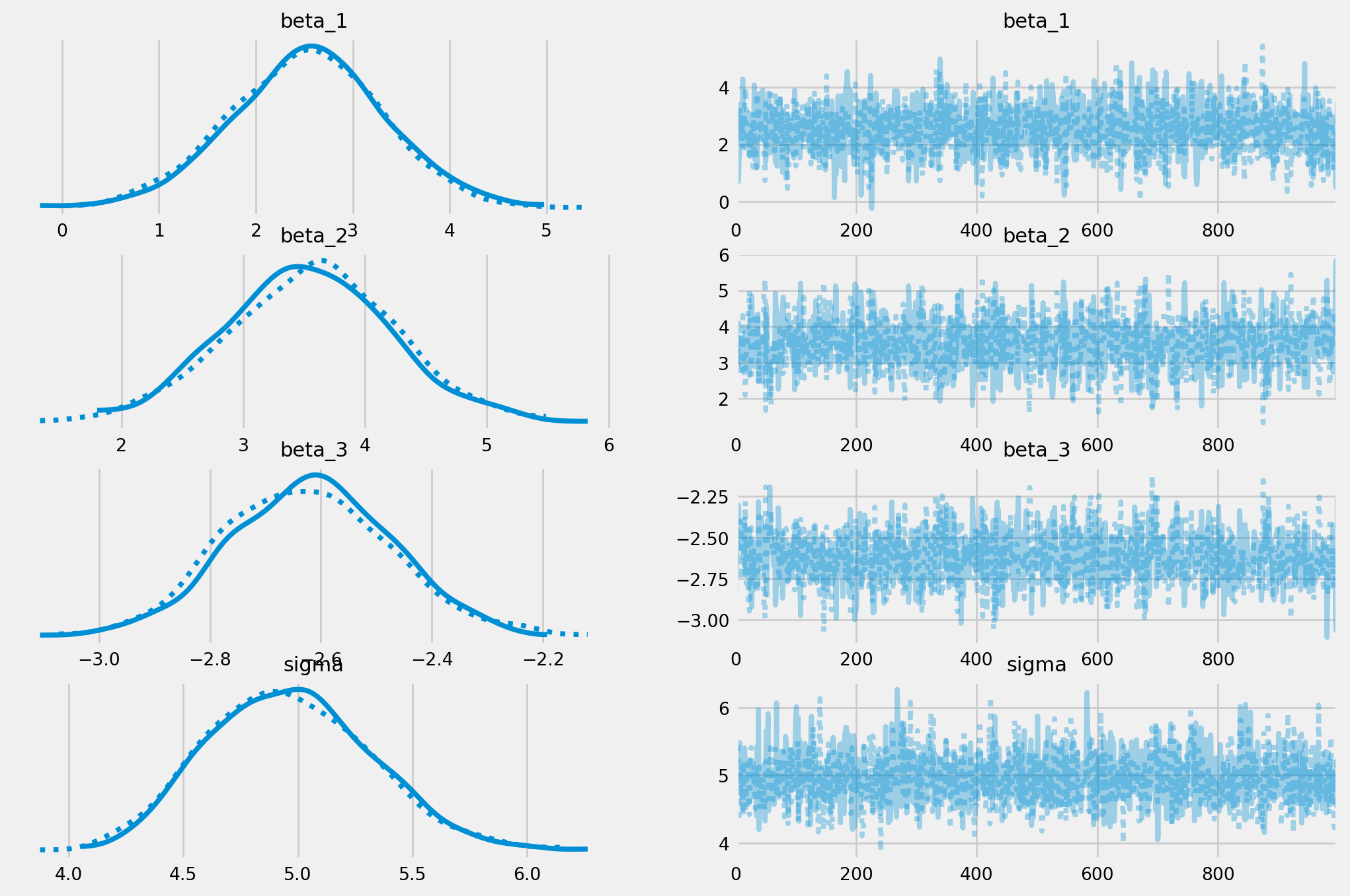
Auto-assigning NUTS sampler...
Initializing NUTS using jitter+adapt_diag...
Sequential sampling (2 chains in 1 job)
NUTS: [beta_1, beta_2, beta_3, sigma]

Sampling 2 chains for 1_000 tune and 1_000 draw iterations (2_000 + 2_000 draws total) took 11 seconds.
We recommend running at least 4 chains for robust computation of convergence diagnostics

az.plot_trace(trace_poly)
plt.show()

beta1_hat_mu = np.mean(trace_poly.posterior.beta_1.values[0])
beta2_hat_mu = np.mean(trace_poly.posterior.beta_2.values[0])
beta3_hat_mu = np.mean(trace_poly.posterior.beta_3.values[0])
Y_hat = beta1_hat_mu + beta2_hat_mu * X + beta3_hat_mu * X**2

beta_1, beta_2, beta_3 = 2, 5, -3
fig, ax = plt.subplots(figsize=(8, 8))
ax.plot(
    X,
    Y_mu,
    color="tomato",
    label=r"True: $Y={}+{}X_2{}X_3^2$".format(beta_1, beta_2, beta_3),
)
ax.plot(
    X,
    Y_hat,
    color="DarkSlateBlue",
    lw=2,
    ls="--",
    label=r"Estimated: $Y={:.2f}+{:.2f}X_2{:.2f}X_3^2$".format(
        beta1_hat_mu, beta2_hat_mu, beta3_hat_mu
    ),
)
ax.scatter(X, Y, marker="1")
ax.legend()
plt.show()